| GEATbx: | Main page Tutorial Algorithms M-functions Parameter/Options Example functions www.geatbx.com |
You are faced with a new optimization problem. How are you best going to approach this task? What questions have to be asked? What do you have to consider? What aspects do you have to examine?
In this section I attempt to provide step-by-step instructions for solving optimization problems. Every single step is illustrated with examples, and you will find cross-references to other sections offering further examples.
The approach I am presenting here is based on my own experiences gained in the course of solving real-world optimization problems using the GEATbx. I have received lots of positive feedback from many others who found this approach helpful for solving complex problems.
The main points are:
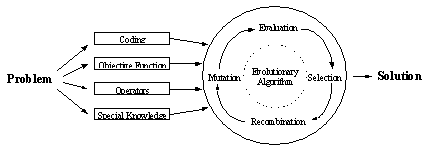
Fig. 9-1 illustrates these points. The first thing to do when confronted with a new problem is to analyze it. This will provide you with the coding, number and boundaries of variables. Now you can implement the objective function. Very often you will have to gather further information on the system behavior. Once you have a basic understanding of the system you can start selecting operators and parameters of the evolutionary algorithm. With this information you have the foundation to start executing the optimization.
Fig. 9-1. Procedure for solving optimization problems using evolutionary algorithms
Some of these steps can be utilized with other optimization tools or methods as well. Additionally, I have included several alternatives to investigating the system behavior. These help gain further information about the problem and can also be applied without optimization. These tools are mostly included in the GEATbx.
9.1 Classifying the Problem and Defining the Objective Function |
|
When you begin to work on a new application you first need to classify the optimization problem. Consider how the system you want to investigate is defined and which outbound interfaces exist or have to be defined. This means you have to determine:
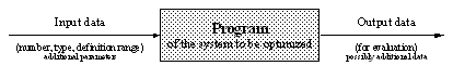
The system has to be available as a program which is entirely controlled through the input data (and possibly the additional parameters) and which as the result of the execution provides the output data. This program is the implementation of the objective function. Fig. 9-2 represents this structure graphically.
Fig. 9-2. Structure of the system to be optimized as objective function
The objective function is not only applicable within the optimization. It can also be applied during program/system simulation with input data, e.g.:
It is very important that the objective function is implemented to be universally applicable to all these areas of application! You will find that using just one program for the problem at hand (optimization, problem-specific visualization, single simulation) pays off and also facilitates program maintenance.
9.2 Investigating the System Behavior |
|
The basic questions when beginning to work on a new problem are: what are the system properties or, for that matter, the objective function properties, what does the search space look like, and do specific features occur. Often these questions only crop up once the first optimization has been carried out and the hoped for results have not been obtained.
The results of the investigations suggested in the following could offer new information on the system behavior as well as indicate the type of objective function and the optimization procedure needed for a successful optimization.
The system at hand generally poses a high-dimensional problem for the optimization. An objective function value, subject to the given parameters, is returned as result of the simulation and application of the objective function.
The generally applicable investigations of the system behavior can be subdivided as follows:
I will take a closer look at these areas in the following.
The systems under test are mostly high-dimensional (more than five dimensions or five parameters). That is why a direct graphic representation of the search space is not possible. However, it is possible to illustrate some features of the objective function by creating one or two-dimensional slices. The results of slicing can be visualized using standard diagrams.
The slices through the objective function are made through a certain point in the search space (here called center point). To calculate the slices through the center point all non-varying parameters of the system are kept constant to the values of the center point. The varying or free parameters are changed within an area around the center point. The boundaries of this area determine the extent of the slices as well as the level of detail. The area around the center point is discretized, the corresponding objective function values calculated, and the results visualized in 2-D and 3-D graphics.
The center point can be the result of an optimization and thus represent a very good point, or it can be a point of great importance within the search domain.
As the standard visualization methods are limited to three dimensions, only one-dimensional (variation of one parameter) and two-dimensional slices (variation of two parameters) can be carried out. One-dimensional slices are easy to calculate. But they can only offer information along the coordinate axis of this one varied parameter. Two-dimensional slices need clearly more calculations, however, they offer additional information about the interaction/correlation between the two varied parameters.
The following information can be deduced from the slices through the objective function:
However, keep in mind that all information drawn from these slices is only valid for the represented area and subject to restrictions. Due to the oftentimes non-linear relations between parameters it is possible to deduce different information for different areas. The gathered information is thus only valid for the examined areas. The results may be valid for other areas too, however this need not be the case.
For the parameter optimization of different real-world systems, variational diagrams were used for investigating the system behavior. Currently they are only explained in detail in Chapter 8 of [Poh99b] (greenhouse control system, car steering example).
Most of the commonly used techniques for visualization are limited to representing data depending on one or two variables. This is due to the human visual limitation to three dimensions. There are two possible extensions to go beyond this limitation: using color for the fourth dimension and time as the fifth dimension. Neither possibility is very common and requires practice, especially if time is used for visualizing the fifth dimension. However, if the problem incorporates more than five dimensions a new method for visualizing arbitrarily high dimensions must be found.
For the visualization of multi-dimensional data a method to transform multi-dimensional data to a lower dimension is needed, preferably to 2 or 3 dimensions. This transformation should provide a lower-dimensional picture where the dissimilarities between the data points of the multi-dimensional domain corresponds with the dissimilarities of the lower-dimensional domain.
These transformation methods are referred to as multi-dimensional scaling. One well-known multi-dimensional scaling method is the Sammon-Mapping method [Sam69].
Please note that all these procedures are subject to information loss. On the one hand, visualization of the information is only possible in this way. On the other hand, we have to take the reduction of information into consideration when interpreting the results.
The multi-dimensional visualization can be applied to the following tasks:
The first four tasks can be calculated and subsequently visualized with the aid of functions which are included in the GEATbx. Currently, the last variant still comes across calculation and visualization problems. Even for an objective function with only ten dimensions or variables large data amounts have to be processed.
These methods enable a clear illustration of complex data relations where other methods either fail or require a great deal of time and familiarization.
An important aspect of investigating new systems is the analysis of the size/dimensionality of the problem and the possible means of its reduction. Most real-world systems are high-dimensional. Often, it is possible to reduce the number of dimensions for the optimization without distorting the results. If this is not directly possible try and perform first optimizations with a reduced or limited system to obtain a better impression of the overall system behavior.
Which variants of dimension reduction or difficulties should you examine?
A few examples of the GEATbx apply the above mentioned methods. Currently they are only explained in detail in Chapter 8 of [Poh99b] (greenhouse control system, car steering example).
9.3 Selecting the Optimization Method |
|
With our knowledge of the type of the system at hand and the findings of the preliminary examination on the system behavior (Section. 9.2) we now have to choose an optimization method. This can be a single method, or a combination of several methods, or variants of one or more methods.
The number of different problem classes is huge, and for each problem class a different method might be most suitable.
Chapter 'Combination of Operators and Options to Produce Evolutionary Algorithms' in "GEATbx Introduction" deals with the selection procedure of methods and operators as well as the specification of appropriate options/parameters. Section 'Generally Adjustable Operators and Options' in "GEATbx Introduction" gives you indications on methods and operators which can be used for most problem classes. Section 'Globally Oriented Parameter Optimization' in "GEATbx Introduction" onwards deals with the definition of optimization methods for special problem classes. All suggestions are based on my own experiences and my work on different systems as well as on results found in the literature.
9.4 Executing and Evaluating Optimizations |
|
Once you have selected one or more optimization methods, first optimizations can be carried out. These can already provide information on how easily the problem can be solved.
Should the first trials already provide the optimal solution (with knowledge of the optimum) or a good or sufficient result, we can consider the problem as solved. Of course, depending on further requirements it is also possible to apply the methods described in the following to find the solutions even more easily.
More often than not, a problem cannot be considered solved after the first runs. Either the results are unsatisfactory or, if the optimum is not known, there is no way of being certain about the obtained results. This is where you should start to find methods which are better suited.
Basically, there are two approaches: either different methods, operators or options are used, or the number of individuals and/or sub-populations is increased. The latter procedure leads to a clear increase in calculation time because the number of individuals linearly effects the overall calculation time (at least in most real problems). If the total calculation time is still less than 24 hours it at least resolves the question as to what extent it is possible to find a solution in this way.
Should the methods used so far prove unsuccessful new variants have to be found. At this point it is necessary to reconsider the system properties. If the system cannot be optimized the way we had hoped for the system must have properties which have not been included in the selection process. By applying further methods it is possible to obtain additional information about the problem at hand.
The visualization possibilities can be an important help when evaluating executed runs. These permit a detailed insight into the state of the population during various stages in an optimization as well as the course of the optimization. Questions as to an early convergence of the population, the existence of several extreme values, or the curve of variables of good individuals find answers here. You need to familiarize yourself with the application of these methods in order to be able to interpret the diagrams. The visualization methods offer the best possible insight into the current state and course of the optimization process and open up new means to adapt the parameters used in the optimization procedure. You can find examples of their application in the following Sections.
At this point I would like to refer to the simultaneous application of different strategies during an optimization run. Please see Chapter 'Application of different strategies' in "GEATbx Introduction" for more details. This procedure on the one hand enables you to apply more than one strategy to solve a problem. On the other hand, it is often the case that, in dependence of the progress of the optimization, different methods are better suited for different stages within the optimization run. The strategies thus support each other, i.e. the success of one strategy enables the subsequent success of another one.
One good example to illustrate this is the application of several mutation variants, where one variant performs a rough search, another one a more refined search, and yet another one an even more refined search. A similar process can be achieved by the simultaneous use of different recombination operators. During the subsequent evaluation it can very easily be checked at what time which of the applied strategies was successful. These means enable us to find the most promising methods for solving a problem. These can in turn be further refined to solve the problem at hand in the best possible and least time-consuming way.
If you find that after having applied the existing and known methods the results are still unsatisfactory you have to consider including further problem-specific knowledge. For example:
The first two points should always be applied, in case this knowledge is available. This usually leads to a clear reduction of the search domain and consequently to an acceleration of finding satisfactory results. The development of special operators is usually very difficult and has, as far as current problems go, not been necessary.
The methods I have introduced for solving optimization problems and the represented variables should make it possible to solve many occurring engineering problems. You need more time to become familiar with bigger and more complex problems. The problem has to be examined closely during different optimization trials. Once the methods and means have been found to solve the problem we have often also obtained new knowledge on the system which was not known even to the experts before the optimization. The optimization process examines such areas of the system which were not taken into consideration beforehand. This increase in knowledge should not be underestimated, neither by the experts of the system to be optimized, nor the system engineer who executes the optimization.
If, after having occupied yourself extensively with the system, you find that the method of evolutionary algorithms seems most appropriate, use it. However, if a problem can be solved with a special method (e.g. gradient based methods) this means that a solution will usually be found more quickly than by using evolutionary algorithms. However, these special methods often require system properties which are hardly guaranteed in real systems (rectangular shapes, differentiability, etc.). In these cases, evolutionary algorithms offer a large spectrum of efficient strategies and operators for solving the optimization problem.

| GEATbx: | Main page Tutorial Algorithms M-functions Parameter/Options Example functions www.geatbx.com |