| GEATbx: | Main page Tutorial Algorithms M-functions Parameter/Options Example functions www.geatbx.com |
In selection the offspring producing individuals are chosen. The first step is fitness assignment. Each individual in the selection pool receives a reproduction probability depending on the own objective value and the objective value of all other individuals in the selection pool. This fitness is used for the actual selection step afterwards.
Throughout this section some terms are used for comparing the different selection schemes. The definition of these terms follow [Bak87] and [BT95].
selective pressure
bias:
spread
loss of diversity
selection intensity
selection variance
3.1 Rank-based fitness assignment |
|
In rank-based fitness assignment, the population is sorted according to the objective values. The fitness assigned to each individual depends only on its position in the individuals rank and not on the actual objective value.
Rank-based fitness assignment overcomes the scaling problems of the proportional fitness assignment. (Stagnation in the case where the selective pressure is too small or premature convergence where selection has caused the search to narrow down too quickly.) The reproductive range is limited, so that no individuals generate an excessive number of offspring. Ranking introduces a uniform scaling across the population and provides a simple and effective way of controlling selective pressure.
Rank-based fitness assignment behaves in a more robust manner than proportional fitness assignment and, thus, is the method of choice. [BH91], [Why89]
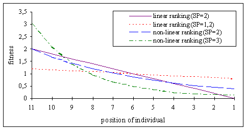
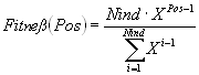
Consider Nind the number of individuals in the population, Pos the position of an individual in this population (least fit individual has Pos=1, the fittest individual Pos=Nind) and SP the selective pressure. The fitness value for an individual is calculated as:
Linear ranking:
Linear ranking allows values of selective pressure in [1.0, 2.0].
A new method for ranking using a non-linear distribution was introduced in [Poh95]. The use of non-linear ranking permits higher selective pressures than the linear ranking method.
Non-linear ranking:
X is computed as the root of the polynomial:
(3-3)
Non-linear ranking allows values of selective pressure in [1, Nind - 2].
Figure compares linear and non-linear ranking graphically.
Fig. 3-1: Fitness assignment for linear and non-linear ranking
The probability of each individual being selected for mating depends on its fitness normalized by the total fitness of the population.
Table contains the fitness values of the individuals for various values of the selective pressure assuming a population of 11 individuals and a minimization problem.
Table 3-1: Dependency of fitness value from selective pressure
fitness value (parameter: selective pressure) | |||||
linear ranking |
no ranking |
non-linear ranking | |||
objective value |
2.0 |
1.1 |
1.0 |
3.0 |
2.0 |
1 |
2.0 |
1.10 |
1,0 |
3.00 |
2.00 |
3 |
1.8 |
1.08 |
1,0 |
2.21 |
1.69 |
4 |
1.6 |
1.06 |
1,0 |
1.62 |
1.43 |
7 |
1.4 |
1.04 |
1,0 |
1.99 |
1.21 |
8 |
1.2 |
1.02 |
1,0 |
0.88 |
1.03 |
9 |
1.0 |
1.00 |
1,0 |
0.65 |
0.87 |
10 |
0.8 |
0.98 |
1,0 |
0.48 |
0.74 |
15 |
0.6 |
0.96 |
1,0 |
0.35 |
0.62 |
20 |
0.4 |
0.94 |
1,0 |
0.26 |
0.53 |
30 |
0.2 |
0.92 |
1,0 |
0.19 |
0.45 |
95 |
0.0 |
0.90 |
1,0 |
0.14 |
0.38 |
In [BT95] an analysis of linear ranking selection can be found.
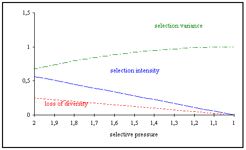
Fig. 3-2: Properties of linear ranking
Selection intensity
(3-4)
Loss of diversity
(3-5)
Selection variance
(3-6)
3.2 Multi-objective Ranking |
|
Where proportional and rank-based fitness assignment is concerned it is assumed that individuals display only one objective function value. In many real world problems, however, there are several criteria which have to be considered in order to evaluate the quality of an individual. Only on the basis of the comparison of these several criteria (thus multi-objective) can a decision be made as to the superiority of one individual over another. Then, as in single-objective problems, an order of individuals within the population can be established from these reciprocal comparisons - multi-objective ranking. After this order has been established the single-objective ranking methods from the subsection 3.1 can be used to convert the order of the individuals to corresponding fitness values.
Multi-objective fitness assignment (and with it multi-objective optimization ) is concerned with the simultaneous minimization of NObj criteria fr, with r = 1, ..., NObj. The values fr are determined by the objective function, which in turn is dependent on the variables of the individuals (the decision variables).
A straightforward example should serve as the motivation for the following considerations. When objects are produced, the production costs should be kept low and the objects should be produced quickly. Various solutions can be developed during production planning which may differ regarding the number and type of the machines employed, as well as regarding the number of workers. The criteria production costs f1 and production time f2, both of which are determined by the objective function, serve as evaluation criteria for each solution.
The superiority of one solution over the other can be decided by comparing 2 solutions. It can be carried out both generally and for as many criteria as desired, following the schema in equation 3-7.
PARETO-ranking resp. PARETO-dominance:
If solution1 is p< (partially less than) solution2, it follows that solution1 dominates solution2. In the example used here this means: if costs and time are less for solution1 than for solution2, it follows that solution1 is superior to solution2. It would even be sufficient if one of the two values was equal for both solutions (equal costs) and only the other value was lower (less time).
If, however, none of the solutions dominates the other both solutions are to be regarded as equivalent with respect to the PARETO-order. The same rank is assigned to individuals which do not dominate each other.
The rank of an individual within the population (ranki) depends on the number of individuals (NumInddominated) dominating this individual [Fon95]:
(3-8)
All solutions that are found during optimization and are not dominated by a different solution constitute the PARETO-optimal solutions (PARETO-optimal set) of this problem (PARETO-optimality). These solutions are assigned a rank value of 1. In the case of each PARETO-optimal solution it is not possible to improve one of the criteria without one or several of the other criteria deteriorating.
When using plain PARETO-ranking in equation 3-7 all PARETO-optimal solutions are equivalent. It is possible, however, to make a further differentiation for many practical problems. As above, the example of object production shall be used to illustrate this. In an extreme case a solution could produce nothing at all. In this case, the costs would equal zero and the production time would be infinite. No other solution could produce the objects at lower costs. Thus, as this solution cannot be dominated, it would belong to the PARETO-optimal solutions if PARETO-dominance was applied exclusively. In a second extreme case a solution could produce objects in a very short time. This would result in very high expenditure, and therefore very high costs. It should be obvious that both cases are not desirable although they belong to the non-dominated solutions which are not dominated.
Goals for the individual criteria can be introduced in order to preclude PARETO-optimal set solutions, which lie outside of the results desired by the user. A solution is only acceptable when the goals for the individual criteria have been reached. This procedure is also termed method of inequalities , MOI, or goal programming. The individual goals are predefined as inequalities.
In the production example used here, this could mean that an upper limit for costs and production time is determined. The result is not acceptable until both goals are simultaneously reached or fallen short of by means of a solution.
When the goals are included in the multi-objective ranking the comparison of two solutions becomes somewhat more complex. The following assumptions are made:
(3-9)
In the definitions the operator partially less p< from equation 3-7 is used for each of the following definitions. It is possible to distinguish 3 different cases.
1. Solution1 does not fulfill any goals:
(3-10)
2. Solution1 fulfills all goals:
(3-11)
3. Solution1 fulfills some goals:
(3-12)
PARETO-ranking using a vector of goals for the individual criteria, allows for an improved generation of the sequence of a number of solutions compared to plain PARETO-ranking.
Multi-objective optimization is carried out in order to find a number of non-dominated solutions, the PARETO-optimal set. A normal evolutionary algorithm, however, converges at a single solution. This process is termed a genetic drift. For this reason, methods must be built in, which achieve the maintenance or expansion of population diversity (prevention of premature convergence).
On the one hand, the genetic drift can be counteracted by the application of fitness sharing). On the other hand, the algorithm has the effect that a greater part of the pareto-optimal solution is ascertained. The basic principle is that individuals in a particular niche must share the resources available amongst themselves. In this way, the more individuals are near an individual, the lower its fitness becomes.
During application the size of the niches and the allocation of resources within each niche must be established. Methods for fitness sharing are suggested in [HN93], [SD94] and [Fon95],amongst others.
In this subsection it was only possible to provide a short introduction to the multi-objective fitness assignment within the context of evolutionary algorithms. The relevant literature should be referred to for more specific questions regarding individual procedures: [Hor97], [Fon95], [ZT98], [HN93], [SD94], [Vel99]. A list of a large amount of literature on multi-objective optimization with evolutionary algorithms can be accessed in [Coe99]. There is a great deal of literature on multi-objective optimization not specific to the evolutionary algorithm. [Mie99] is recommended as a good starting point.
When considering different methods and component parts used for multi-objective optimization one should not forget classic methods for the integration of several criteria (scalarization method, also called aggregation of objectives).
The weighted sum is the most well-known method. Here each criterion is assigned a weighting value. By means of the linear combination of all the weighted criteria a combined objective function value Fws is achieved:
(3-13)
The weighted sum is especially used in cases when the varying significance of the individual criteria is known or can be estimated. As this is frequently the case where practical application is concerned, the weighted sum is often applied.
If a multi-objective problem is solved by means of single-objective optimization, only a point solution is obtained. The advantage of obtaining several solutions of equal value relating to a target vector is lost. At this stage the user must decide whether the simple use of the weighted sum or the approximation of the PARETO-optimal solutions is more important for the solution of the problem.
3.3 Roulette wheel selection |
|
The simplest selection scheme is roulette-wheel selection, also called stochastic sampling with replacement [Bak87]. This is a stochastic algorithm and involves the following technique:
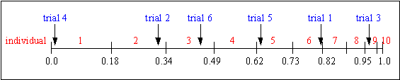
The individuals are mapped to contiguous segments of a line, such that each individual's segment is equal in size to its fitness. A random number is generated and the individual whose segment spans the random number is selected. The process is repeated until the desired number of individuals is obtained (called mating population). This technique is analogous to a roulette wheel with each slice proportional in size to the fitness, see figure .
Table shows the selection probability for 11 individuals, linear ranking and selective pressure of 2 together with the fitness value. Individual 1 is the most fit individual and occupies the largest interval, whereas individual 10 as the second least fit individual has the smallest interval on the line (see figure ). Individual 11, the least fit interval, has a fitness value of 0 and get no chance for reproduction
Table 3-2: Selection probability and fitness value
Number of individual |
1 |
2 |
3 |
4 |
5 |
6 |
7 |
8 |
9 |
10 |
11 |
fitness value |
2.0 |
1.8 |
1.6 |
1.4 |
1.2 |
1.0 |
0.8 |
0.6 |
0.4 |
0.2 |
0.0 |
selection probability |
0.18 |
0.16 |
0.15 |
0.13 |
0.11 |
0.09 |
0.07 |
0.06 |
0.03 |
0.02 |
0.0 |
For selecting the mating population the appropriate number of uniformly distributed random numbers (uniform distributed between 0.0 and 1.0) is independently generated.
sample of 6 random numbers:
0.81, 0.32, 0.96, 0.01, 0.65, 0.42.
Figure shows the selection process of the individuals for the example in table together with the above sample trials.
Fig. 3-3: Roulette-wheel selection
After selection the mating population consists of the individuals:
1, 2, 3, 5, 6, 9.
The roulette-wheel selection algorithm provides a zero bias but does not guarantee minimum spread.
3.4 Stochastic universal sampling |
|
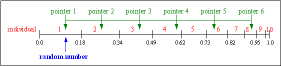
Stochastic universal sampling [Bak87] provides zero bias and minimum spread. The individuals are mapped to contiguous segments of a line, such that each individual's segment is equal in size to its fitness exactly as in roulette-wheel selection. Here equally spaced pointers are placed over the line as many as there are individuals to be selected. Consider NPointer the number of individuals to be selected, then the distance between the pointers are 1/NPointer and the position of the first pointer is given by a randomly generated number in the range [0, 1/NPointer].
For 6 individuals to be selected, the distance between the pointers is 1/6=0.167. Figure shows the selection for the above example.
sample of 1 random number in the range [0, 0.167]:
0.1.
Fig. 3-4: Stochastic universal sampling
After selection the mating population consists of the individuals:
1, 2, 3, 4, 6, 8.
Stochastic universal sampling ensures a selection of offspring which is closer to what is deserved then roulette wheel selection.
3.5 Local selection |
|
In local selection every individual resides inside a constrained environment called the local neighborhood. (In the other selection methods the whole population or subpopulation is the selection pool or neighborhood.) Individuals interact only with individuals inside this region. The neighborhood is defined by the structure in which the population is distributed. The neighborhood can be seen as the group of potential mating partners.
Local selection is part of the local population model, see Section 7.2.
The first step is the selection of the first half of the mating population uniform at random (or using one of the other mentioned selection algorithms, for example, stochastic universal sampling or truncation selection). Now a local neighborhood is defined for every selected individual. Inside this neighborhood the mating partner is selected (best, fitness proportional, or uniform at random).
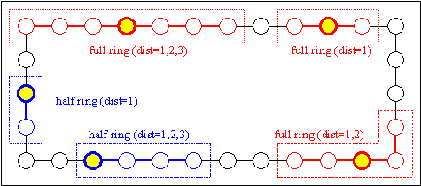
The structure of the neighborhood can be:
Fig. 3-5: Linear neighborhood: full and half ring
The distance between possible neighbors together with the structure determines the size of the neighborhood. Table gives examples for the size of the neighborhood for the given structures and different distance values.
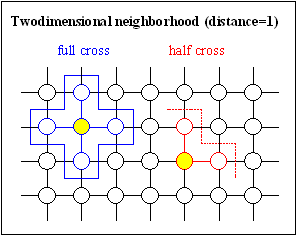
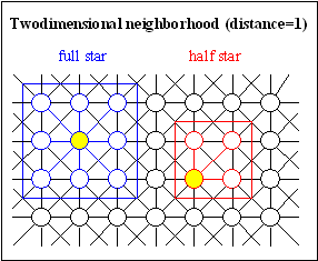
Fig. 3-6: Two-dimensional neighborhood; left: full and half cross, right: full and half star
Between individuals of a population an `isolation by distance' exists. The smaller the neighborhood, the bigger the isolation distance. However, because of overlapping neighborhoods, propagation of new variants takes place. This assures the exchange of information between all individuals.
The size of the neighborhood determines the speed of propagation of information between the individuals of a population, thus deciding between rapid propagation or maintenance of a high diversity/variability in the population. A higher variability is often desired, thus preventing problems such as premature convergence to a local minimum. Similar results were drawn from simulations in [VBS91]. Local selection in a small neighborhood performed better than local selection in a bigger neighborhood. Nevertheless, the interconnection of the whole population must still be provided. Two-dimensional neighborhood with structure half star using a distance of 1 is recommended for local selection. However, if the population is bigger (>100 individuals) a greater distance and/or another two-dimensional neighborhood should be used.
Tab. 3-3: Number of neighbors for local selection
distance | ||
structure of selection |
1 |
2 |
full ring |
2 |
4 |
half ring |
1 |
2 |
full cross |
4 |
8 (12) |
half cross |
2 |
4 (5) |
full star |
8 |
24 |
half star |
3 |
8 |
3.6 Truncation selection |
|
Compared to the previous selection methods modeling natural selection truncation selection is an artificial selection method. It is used by breeders for large populations/mass selection.
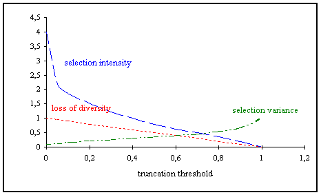
In truncation selection individuals are sorted according to their fitness. Only the best individuals are selected for parents. These selected parents produce uniform at random offspring. The parameter for truncation selection is the truncation threshold Trunc. Trunc indicates the proportion of the population to be selected as parents and takes values ranging from 50%-10%. Individuals below the truncation threshold do not produce offspring. The term selection intensity is often used in truncation selection. Table shows the relation between both.
Tab. 3-4: Relation between truncation threshold and selection intensity
truncation threshold |
1% |
10% |
20% |
40% |
50% |
80% |
selection intensity |
2.66 |
1.76 |
1.2 |
0.97 |
0.8 |
0.34 |
In [BT95] an analysis of truncation selection can be found. The same results have been derived in a different way in [CK70] as well.
Selection intensity
(3-14)
Loss of diversity
(3-15)
Selection variance
(3-16)
Fig. 3-7: Properties of truncation selection
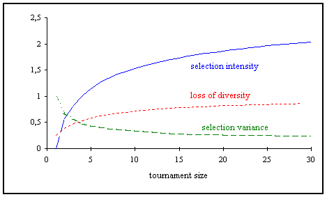
3.7 Tournament selection |
|
In tournament selection [GD91] a number Tour of individuals is chosen randomly from the population and the best individual from this group is selected as parent. This process is repeated as often as individuals must be chosen. These selected parents produce uniform at random offspring. The parameter for tournament selection is the tournament size Tour. Tour takes values ranging from 2 to Nind (number of individuals in population). Table and figure show the relation between tournament size and selection intensity [BT95].
Tab. 3-5: Relation between tournament size and selection intensity
tournament size |
1 |
2 |
3 |
5 |
10 |
30 |
selection intensity |
0 |
0.56 |
0.85 |
1.15 |
1.53 |
2.04 |
In [BT95] an analysis of tournament selection can be found.
Selection intensity
(3-17)
Loss of diversity
(3-18)
(About 50% of the population are lost at tournament size Tour=5).
Selection variance
Fig. 3-8: Properties of tournament selection
3.8 Comparison of selection schemes |
|
As shown in the previous sections of this chapter the selection methods behave similarly assuming similar selection intensity.
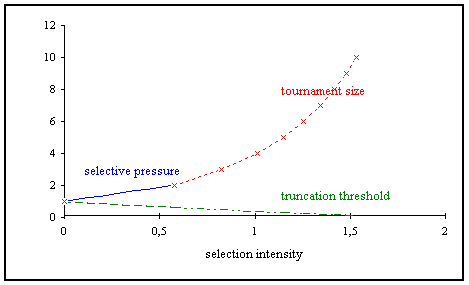
Figure shows the relation between selection intensity and the appropriate parameters of the selection methods (selective pressure, truncation threshold and tournament size). It should be stated that with tournament selection only discrete values can be assigned and linear ranking selection allows only a smaller range for the selection intensity.
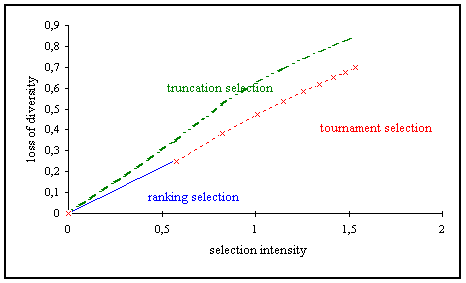
However, the behavior of the selection methods is different. Thus, the selection methods will be compared on the parameters loss of diversity (figure ) and selections variance (figure ) on the selection intensity.
Fig. 3-9: Dependence of selection parameter on selection intensity
Fig. 3-10: Dependence of loss of diversity on selection intensity
Truncation selection leads to a much higher loss of diversity for the same selection intensity compared to ranking and tournament selection. Truncation selection is more likely to replace less fit individuals with fitter offspring, because all individuals below a certain fitness threshold do not have a probability to be selected. Ranking and tournament selection seem to behave similarly. However, ranking selection works in an area where tournament selection does not work because of the discrete character of tournament selection.
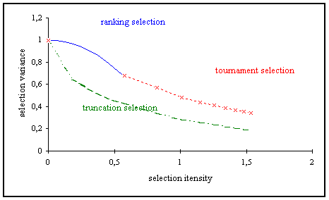
Fig. 3-11: Dependence of selection variance on selection intensity
For the same selection intensity truncation selection leads to a much smaller selection variance than ranking or tournament selection. As can be seen clearly ranking selection behaves similar to tournament selection. However, again ranking selection works in an area where tournament selection does not work because of the discrete character of tournament selection. In [BT95] was proven that the fitness distribution for ranking and tournament selection for SP=2 and Tour=2 (SelInt=1/sqrt(pi)) is identical.

| GEATbx: | Main page Tutorial Algorithms M-functions Parameter/Options Example functions www.geatbx.com |


 (
(