

Recombination produces new individuals in combining the information contained in two or more parents (parents - mating population). This is done by combining the variable values of the parents. Depending on the representation of the variables different methods must be used.
Section 4.1 describes the discrete recombination. This method can be applied to all variable representations. Section 4.2 explains methods for real valued variables. Methods for binary valued variables are described in Section 4.3.
The methods for binary valued variables constitute special cases of the discrete recombination. These methods can all be applied to integer valued and real valued variables as well.
4.1 All representations - Discrete recombination |
Discrete recombination [MSV93a] performs an exchange of variable values between the individuals. For each position the parent who contributes its variable to the offspring is chosen randomly with equal probability.
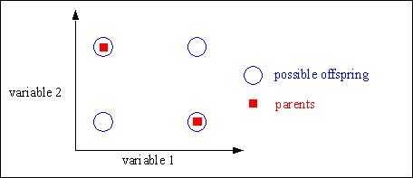
Discrete recombination generates corners of the hypercube defined by the parents. Figure shows the geometric effect of discrete recombination.
Fig. 4-1: Possible positions of the offspring after discrete recombination

Consider the following two individuals with 3 variables each (3 dimensions), which will also be used to illustrate the other types of recombination for real valued variables:
individual 1      12     25      5
 individual 2     123      4     34
For each variable the parent who contributes its variable to the offspring is chosen randomly with equal probability.:
sample 1           2      2      1
 sample 2           1      2      1
After recombination the new individuals are created:
offspring 1      123      4      5
 offspring 2       12      4      5
Discrete recombination can be used with any kind of variables (binary, integer, real or symbols).
4.2 Real valued recombination |
The recombination methods in this section can be applied for the recombination of individuals with real valued variables.
Intermediate recombination [MSV93a] is a method only applicable to real variables (and not binary variables). Here the variable values of the offspring are chosen somewhere around and between the variable values of the parents.
Offspring are produced according to the rule:
where a is a scaling factor chosen uniformly at random over an interval [-d, 1+d] for each variable anew.
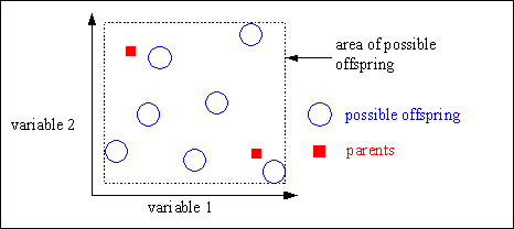
The value of the parameter d defines the size of the area for possible offspring. A value of d = 0 defines the area for offspring the same size as the area spanned by the parents. This method is called (standard) intermediate recombination. Because most variables of the offspring are not generated on the border of the possible area, the area for the variables shrinks over the generations. This shrinkage occurs just by using (standard) intermediate recombination. This effect can be prevented by using a larger value for d. A value of d = 0.25 ensures (statistically), that the variable area of the offspring is the same as the variable area spanned by the variables of the parents. See figure 4-2 for a picture of the area of the variable range of the offspring defined by the variables of the parents.
Fig. 4-2: Area for variable value of offspring compared to parents in intermediate recombination

Consider the following two individuals with 3 variables each:
individual 1      12     25      5
 individual 2     123      4     34
The chosen a for this example are:
sample 1         0.5    1.1   -0.1
 sample 2         0.1    0.8    0.5
The new individuals are calculated as:
offspring 1     67.5    1.9    2.1
 offspring 2     23.1    8.2   19.5
Intermediate recombination is capable of producing any point within a hypercube slightly larger than that defined by the parents. Figure 4-3 shows the possible area of offspring after intermediate recombination.
Fig. 4-3: Possible area of the offspring after intermediate recombination

Line recombination [MSV93a] is similar to intermediate recombination, except that only one value of a for all variables is used. The same a is used for all variables:
For the value of d the statements given for intermediate recombination are applicable.
Consider the following two individuals with 3 variables each:
individual 1      12     25      5
 individual 2     123      4     34
The chosen Alpha for this example are:
sample 1         0.5
 sample 2         0.1
The new individuals are calculated as:
offspring 1     67.5   14.5   19.5
 offspring 2     23.1   22.9    7.9
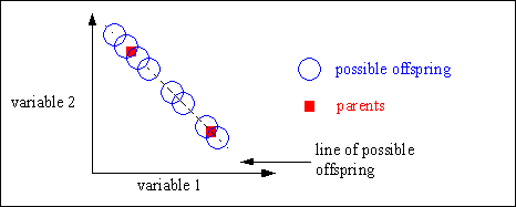
Line recombination can generate any point on the line defined by the parents. Figure 4-4 shows the possible positions of the offspring after line recombination.
Fig. 4-4: Possible positions of the offspring after line recombination

Extended line recombination [Müh94] generates offspring on a line defined by the variable values of the parents. However, extended line recombination is not restricted to the line between the parents and a small area outside. The parents just define the line where possible offspring may be created. The size of the area for possible offspring is defined by the domain of the variables.
Inside this possible area the offspring are not uniform at random distributed. The probability of creating offspring near the parents is high. Only with low probability offspring are created far away from the parents. If the fitness of the parents is available, then offspring are more often created in the direction from the worse to the better parent (directed extended line recombination).
Offspring are produced according to the following rule:
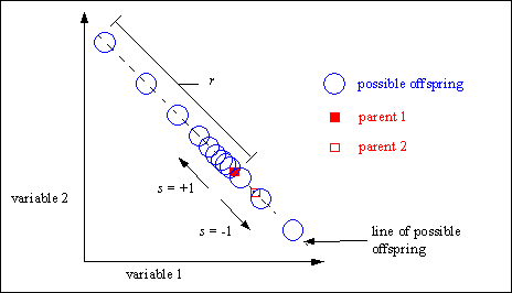
The creation of offspring uses features similar to the mutation operator for real valued variables (see Section 5.1). The parameter a defines the relative step-size, the parameter r the maximum step-size and the parameter s the direction of the recombination step.
Figure 4-5 tries to visualize the effect of extended line recombination.
The parameter k determines the precision used for the creation of recombination steps. A larger k produces more smaller steps. For all values of k the maximum value for a is a = 1 (u = 0). The minimum value of a depends on k and is a =2-k (u = 1). Typical values for the precision parameter k are in the area from 4 to 20.
Fig. 4-5: Possible positions of the offspring after extended line recombination according to the positions of the parents and the definition area of the variables

A robust value for the parameter r (range of recombination step) is 10% of the domain of the variable. However, according to the defined domain of the variables or for special cases this parameter can be adjusted. By selecting a smaller value for r the creation of offspring may be constrained to a smaller area around the parents.
If the parameter s (search direction) is set to -1 or +1 with equal probability an undirected recombination takes place. If the probability of s=+1 is higher than 0.5, a directed recombination takes place (offspring are created in the direction from the worse to the better parent - the first parent must be the better parent).
Extended line recombination is only applicable to real variables (and not binary or integer variables).
4.3 Binary valued recombination (crossover) |
This section describes recombination methods for individuals with binary variables. Commonly, these methods are called 'crossover'. Thus, the notion 'crossover' will be used to name the methods.
During the recombination of binary variables only parts of the individuals are exchanged between the individuals. Depending on the number of parts, the individuals are divided before the exchange of variables (the number of cross points). The number of cross points distinguish the methods.
In single-point crossover one crossover position k_[1,2,...,Nvar-1], Nvar: number of variables of an individual, is selected uniformly at random and the variables exchanged between the individuals about this point, then two new offspring are produced. Figure 4-6 illustrates this process.
Consider the following two individuals with 11 binary variables each:
individual 1     0  1  1  1  0  0  1  1  0  1  0
 individual 2     1  0  1  0  1  1  0  0  1  0  1
The chosen crossover position is:
crossover position 5
After crossover the new individuals are created:
offspring 1      0  1  1  1  0| 1  0  0  1  0  1
 offspring 2      1  0  1  0  1| 0  1  1  0  1  0
Fig. 4-6: Single-point crossover

In double-point crossover two crossover positions are selected uniformly at random and the variables exchanged between the individuals between these points. Then two new offspring are produced.
Single-point and double-point crossover are special cases of the general method multi-point crossover.
For multi-point crossover, m crossover positions ki_[1,2,...,Nvar-1], i=1:m, Nvar: number of variables of an individual, are chosen at random with no duplicates and sorted into ascending order. Then, the variables between successive crossover points are exchanged between the two parents to produce two new offspring. The section between the first variable and the first crossover point is not exchanged between individuals. Figure 4-7 illustrates this process.
Consider the following two individuals with 11 binary variables each:
individual 1     0  1  1  1  0  0  1  1  0  1  0
 individual 2     1  0  1  0  1  1  0  0  1  0  1
The chosen crossover positions are:
cross pos. (m=3) 2 6 10
After crossover the new individuals are created:
offspring 1      0  1| 1  0  1  1| 0  1  1  1| 1
 offspring 2      1  0| 1  1  0  0| 0  0  1  0| 0
Fig. 4-7: Multi-point crossover

The idea behind multi-point, and indeed many of the variations on the crossover operator, is that parts of the chromosome representation that contribute most to the performance of a particular individual may not necessarily be contained in adjacent substrings [Boo87]. Further, the disruptive nature of multi-point crossover appears to encourage the exploration of the search space, rather than favouring the convergence to highly fit individuals early in the search, thus making the search more robust [SDJ91b].
Single and multi-point crossover define cross points as places between loci where an individual can be split. Uniform crossover [Sys89] generalizes this scheme to make every locus a potential crossover point. A crossover mask, the same length as the individual structure is created at random and the parity of the bits in the mask indicate which parent will supply the offspring with which bits. This method is identical to discrete recombination, see Section 4.1.
Consider the following two individuals with 11 binary variables each:
individual 1     0  1  1  1  0  0  1  1  0  1  0
 individual 2     1  0  1  0  1  1  0  0  1  0  1
For each variable the parent who contributes its variable to the offspring is chosen randomly with equal probability. Here, the offspring 1 is produced by taking the bit from parent 1 if the corresponding mask bit is 1 or the bit from parent 2 if the corresponding mask bit is 0. Offspring 2 is created using the inverse of the mask, usually.
sample 1         0  1  1  0  0  0  1  1  0  1  0
 sample 2         1  0  0  1  1  1  0  0  1  0  1
After crossover the new individuals are created:
offspring 1      1  1  1  0  1  1  1  1  1  1  1
 offspring 2      0  0  1  1  0  0  0  0  0  0  0
Uniform crossover, like multi-point crossover, has been claimed to reduce the bias associated with the length of the binary representation used and the particular coding for a given parameter set. This helps to overcome the bias in single-point crossover towards short substrings without requiring precise understanding of the significance of the individual bits in the individuals representation. [SDJ91a] demonstrated how uniform crossover may be parameterized by applying a probability to the swapping of bits. This extra parameter can be used to control the amount of disruption during recombination without introducing a bias towards the length of the representation used.
Shuffle crossover [CES89] is related to uniform crossover. A single crossover position (as in single-point crossover) is selected. But before the variables are exchanged, they are randomly shuffled in both parents. After recombination, the variables in the offspring are unshuffled in reverse. This removes positional bias as the variables are randomly reassigned each time crossover is performed.
The reduced surrogate operator [Boo87] constrains crossover to always produce new individuals wherever possible. This is implemented by restricting the location of crossover points such that crossover points only occur where gene values differ.