| GEATbx: | Main page Tutorial Algorithms M-functions Parameter/Options Example functions www.geatbx.com |
The Genetic and Evolutionary Algorithm Toolbox (GEATbx) provides a number of demos. All these functions are called demo*.m (for instance demofun1). The demo-functions provide ready-to-run examples and can be called directly after the installation. All necessary parameters are already set.
2.1 First demonstration |
|
As a first example, run the first demonstration function in Matlab:
demofun1;
This demo defines a number of evolutionary algorithm options, starts the optimization, displays the EA options employed on the screen (see figure 2-1), optimizes the objective function objfun1, returns intermediate information during the optimization in the Matlab command window (see figure 2-2 and 2-4), and visualizes the results graphically every few generations (see figure 2-3). The output on your screen might be slightly different, but the examples below give you a general idea of the output visualization. Below the output figures some of the options inside demofun1 are explained.
Fig. 2-1: Output in Matlab command window at start of optimization run (used options)
Evolutionary Optimization
 Objective function:  objfun1       Date: 22-Dec-2005     Time: 22:12:66
    number of variables:   10
    boundaries of variables:        -512
                                     512
 Evolutionary algorithm parameters:
    subpopulations =      4       individuals =     25   (at start per subpopulation)
    termination    1:  max. generations = 400;
    variable format =    0   (real values - phenotype == genotype)
    selection
          function = selsus
          pressure =    1.7
          gen. gap =    0.9
       reinsertion
              rate =      1
    recombination
          name = recdis  recdis  reclin  recdis
          rate =      1
    mutation
            name = mutreal
            rate =      1
           range =    0.1    0.01   0.001  0.0001
       precision =     16
    regional model
       migration
             rate =   0.1    interval =   20
    output
       results on screen every  5  generation
       grafical display of results every  10  generation
          method = 111111
          style  = 614143
Fig. 2-2: Status information displayed in command window during optimization (some lines removed)
Generation   f-Count     Obj. Function          Term: 1        Time: cpu/gen,  full
     5.           451             40519          [   1.25%]     (  0.00min  00:00:02)
    10.           888             30140          [   2.50%]     (  0.00min  00:00:03)
    15.          1331             12935          [   3.75%]     (  0.00min  00:00:06)
    20.          1776            8572.8          [   5.00%]     (  0.00min  00:00:06)
    25.          2217            4910.8          [   6.25%]     (  0.00min  00:00:08)
    30.          2660            3644.4          [   7.50%]     (  0.00min  00:00:09)
    35.          3100            2414.4          [   8.75%]     (  0.00min  00:00:11)
    40.          3540            1210.6          [  10.00%]     (  0.00min  00:00:11)
    45.          3979            678.95          [  11.25%]     (  0.00min  00:00:13)
    50.          4418            208.31          [  12.50%]     (  0.00min  00:00:14)

   200.         17636       1.1752e-005          [  50.00%]     (  0.00min  00:00:54)
   205.         18076       8.6381e-006          [  51.25%]     (  0.00min  00:00:56)
   210.         18516       8.6179e-006          [  52.50%]     (  0.00min  00:00:57)
   215.         18956       5.6262e-006          [  53.75%]     (  0.00min  00:00:58)
   220.         19396       4.2513e-006          [  55.00%]     (  0.00min  00:00:59)

   370.         32604       4.4879e-008          [  92.50%]     (  0.00min  00:01:38)
   375.         33044       3.9711e-008          [  93.75%]     (  0.00min  00:01:40)
   380.         33484       3.4701e-008          [  95.00%]     (  0.00min  00:01:41)
   385.         33928       3.2459e-008          [  96.25%]     (  0.00min  00:01:42)
   390.         34368       3.1356e-008          [  97.50%]     (  0.00min  00:01:43)
   395.         34808       1.4482e-008          [  98.75%]     (  0.00min  00:01:45)
   400.         35248       1.4482e-008          [ 100.00%]     (  0.00min  00:01:46)
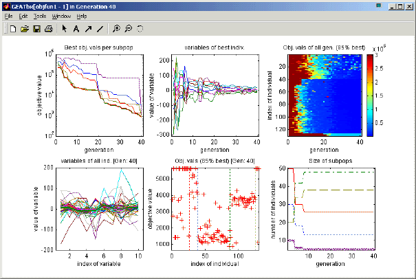
Fig. 2-3: Graphical output during optimization
Fig. 2-4: Result information displayed in command window at the end of the optimization (some parts have been removed)
End of optimization: max. generations (400 generations; 1.78 time minutes)
 Best Objective value:  1.44825e-008   in Generation 393
 Best Individual:   -2.734e-005  -1.4079e-005   2.419e-005 -2.9976e-005
                   -2.8788e-005   9.4641e-005 -1.3272e-005  3.2009e-005
                    2.7127e-005  -1.8188e-005
A number of options are defined in demofun1. Most of these options are not really necessary for a first demo function. However, you can use this function as a template. Let's have a look at some of the options.
The first step provides us with the default parameters for real valued parameters. More information can be found at Predefined Evolutionary Algorithms (in Parameter options).
% Get default parameters for real variables
 GeaOpt = tbx3real;
The second step is to set number of subpopulations (here 5 subpopulations) and number of individuals per subpopulation (here a different number for each subpopulation, 50 individuals for the first subpopulation, 30 individuals in the second subpopulation and so on). Another useful parameter defines, how often textual status information is displayed during an optimization (here every 5 generations).
% Define special parameters
 GeaOpt = geaoptset( GeaOpt ...
            , 'NumberSubpopulation',   5 ...
            , 'NumberIndividuals',   [50, 30, 20, 20, 10] ...
            , 'Output.TextInterval',   5 ...
           );
The definition of the objective function is quite important. Here we use one of the many example objective functions of the GEATbx, objfun1 implementing the hyper sphere function. The objective function is implemented in an m-function. Thus, we simply provide the name of this m-function:
% Define objective function to use
 objfun = 'objfun1';
All the example objective functions of the GEATbx not only contain the definition of the function, but also all the necessary parameters for the application of the function: boundaries of the variables (VLUB: vector of lower and upper bounds), a short textual description, the best objective value (when known), and the corresponding variable values. Thus, the GEATbx can always "ask" the current objective function for the parameters needed. A gateway function to access these parameters is provided.
% Get variable boundaries from objective function
 VLUB = compdiv('getdata_objfun', objfun, 1); % GEATbx v.3.3
 VLUB = geaobjpara(objfun, 1); % GEATbx v.3.4 and newer
A full description of the gateway into the objective functions is given in 'Writing Objective Functions', Chapter 3.
Now all options are defined. Thus, the evolutionary algorithm implemented in geamain2 can be called:
% Start optimization
 [xnew, GeaOpt] = geamain2(objfun, GeaOpt, VLUB);
During the optimization status information and visualization output are displayed on the screen (see figure 2-2, 2-4, and 2-3).
If you want to have a look at the search space of the objective function (visualizing the first 2 dimensions):
% Do a mesh plot of the objective function
 plotmesh(objfun, [-100,-100;100,100]);
2.2 Second demonstration |
|
In order to give an impression of the utility of the GEATbx, a demonstration implementing 3 different evolutionary algorithms and calling many of the example objective functions is provided. Call the demonstration in the Matlab command window:
demogeatbx(1,1);
This call optimizes the objective function objfun1 with a 'Globally oriented optimization (with multiple subpopulations)' nearly identical to the implementation in demofun1.
When the demonstration is called without parameters, you can select one of the available options from a text menu. The first menu provides a selection of at least 16 different objective functions. The second menu offers 3 different evolutionary algorithms (see figure 2-5, bottom).
Fig. 2-5: Demonstration demogeatbx: option selection in menu (top: objective function, bottom: evolutionary algorithm to apply)
» demogeatbx
 --- Please select objective function to use ----
       1) Sphere function (objfun1)
       2) ROSENBROCKs function (objfun2)
       3) RASTRIGINs function (objfun6)
       4) SCHWEFELs function (objfun7)
       5) GRIEWANGKs function (objfun8)
       6) Sum of different power (objfun9)
       7) ACKLEYs path function (objfun10)
       8) LANGERMANNs function (objfun11)
       9) MICHALEWICZs function (objfun12)
       10) Axis parallel ellipsoid (objfun1a)
       11) Rotated ellipsoid (objfun1b)
       12) Moved axis parallel ellipsoid (objfun1c)
       13) Live optimization (objlive1, 2 dim)
       14) Live optimization (objlive1, 10 dim)
       15) FONSECAs MO function 1 (mobjfonseca1)
       16) FONSECAs MO function 2 (mobjfonseca2)
 Select a menu number: 1

 --- Please select the optimization method to use! ----
       1) Globally oriented optimization (multiple subpops)
       2) Globally oriented optimization (1 subpop)
       3) Locally oriented optimization
 Select a menu number: 1
Using this demonstration function you can explore many of the provided objective functions. Each of the objective functions has different properties. Thus, for each objective function the 3 evolutionary algorithms behave differently. For instance, try the following combinations:
demogeatbx(1,2);     demogeatbx(1,3);
 demogeatbx(2,3);     demogeatbx(2,1);
 demogeatbx(12,2);
 demogeatbx(5,1);     demogeatbx(5,3);
The options of the evolutionary algorithms employed are displayed in the Matlab command window at the beginning of the optimization. However, the first 2 evolutionary algorithms ('Globally oriented optimization', most options defined in tbx3real) differ only in the number of subpopulations employed. Both of these use 200 individuals. The third evolutionary algorithm ('Locally oriented optimization') uses an evolution strategy as the mutation operator and no recombination. It works with only 12 individuals. A few other options are also different. Most of the options of this evolutionary algorithm are set inside tbx3es1.
2.3 Your first optimization of an own objective function |
|
Up to now you have only used the demonstration and objective functions provided. It is time to write your first objective function. Let's implement a simple quadratic function with a moved center.
An implementation of the x^2 function with a moved minimum point to [4, 8, 12, ...] is given in figure 2-6. Save these lines in an m-file with the name objexample1.m. Now the objective function is defined.
Fig. 2-6: Definition of objective function objexample1
function ObjVal = objexample1(Chrom)
    % Compute population parameters
    [Nind, Nvar] = size(Chrom);
    % Move the center of the minimum
    Chrom = Chrom - 4 * repmat([1:Nvar], [Nind, 1]);
    % Calculate the objective values
    ObjVal = sum((Chrom .^2)')';
In the command window you can now set a few optimization options before you start the optimization (all other options are taken from the set of default options). These lines can also be written to an m-file creating your own demo example and executing this m-file.
As an example, set the interval of text output to every 3 generations. The second option results in an update of the graphical output every 9 generations. The optimization stops after half a minute (termination method 2 is maximal time in minutes). Using the new objective function and the special options you can call the evolutionary algorithm. Here we also provide the number of variables or dimensions of the objective function (4 variables by defining 4 lowerand 4 upper bounds) and the boundaries of these variables (-50 and 50).
Fig. 2-7: Definition of options, size of the problem (number of variables) and execution of optimization
% Define special parameters
 GeaOpt = geaoptset( 'Output.TextInterval',    3 ...
                   , 'Output.GrafikInterval',  9 ...
                   , 'Termination.MaxTime',  0.5 ...
                   , 'Termination.Method',     2);

 VLUB = [-50,-50,-50,-50; 50,50,50,50];
 geamain2('objexample1', GeaOpt, VLUB)
Using these few lines the optimization is executed and results are shown in the command window (text output) and the graphical result figure. At the end of the run the result is given in the command window (similar to figure 2-4).
The same objective function can easily be optimized for 15 variables/dimensions or more. To do so simply define a larger number of variable boundaries. Now the objective value can only reach a minimum of 140. The boundaries for the higher dimensions do not allow the (unbounded) minimal value to be found. You must therefore call the evolutionary algorithm again with extended/changed boundaries.
Fig. 2-8: Definition of a larger number of variables and with extended boundaries
% Define 15 variables
 VLUB = repmat([-50; 50], [1, 15]);
 geamain2('objexample1', GeaOpt, VLUB)

 % Define different boundaries
 VLUB = repmat([-12; 123], [1, 15]);
 geamain2('objexample1', GeaOpt, VLUB)
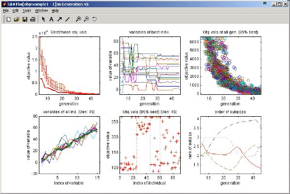
An impression of the graphical output during optimization is given in figure 2-9.
Fig. 2-9: Graphical output during optimization of first own objective function
These are the graphics which default options provided. The top left graph presents the best objective value during the last 40 generations (and the standard deviation of all objective values). The top middle graph visualizes the variables of the best individual over the last 40 generations. Out of the chaos at the beginning, an order seems to emerge and you can try to interpret the results. The top left graph shows all the objective values (to be exact only 85% of the best of each generation) over the last 40 generations. A very interesting graph is presented on the bottom left: all the variables of all the individuals of the current generation. You can clearly see the order in the variable values. The bottom middle graph shows the objective values of the individuals of the current generation and the bottom right graph the order of the subpopulations (both will be explained at a future date).
During optimization the graphical output changes quite substantially. Thus, the graphic in figure 2-9 is just a snapshot. If, however, you follow the changing display during optimization you will soon gain a good insight into the course and the state of the current optimization.
2.4 Further Steps |
|
The examples shown will be sufficient for your first steps using the GEATbx. Have a look at the scripts subdirectory of your geatbx3 installation. This directory contains further demo functions - see the respective help text for more information.
The next step is to learn about 'Writing Objective Functions', see Chapter 3, and how to handle the different 'Variable Representation' in the objective function and the evolutionary algorithm, see Chapter 4.
For an 'Overview of GEA Toolbox Structure' and more information on the 'Calling Tree' of the toolbox, see Chapter 5.

| GEATbx: | Main page Tutorial Algorithms M-functions Parameter/Options Example functions www.geatbx.com |